In this codelab you will train a model to make predictions from numerical data describing a set of cars.
This exercise will demonstrate steps common to training many different kinds of models, but will use a small dataset and a simple (shallow) model. The primary aim is to help you get familiar with the basic terminology, concepts and syntax around training models with TensorFlow.js and provide a stepping stone for further exploration and learning.
Because we are training a model to predict continuous numbers, this task is sometimes referred to as a regression task. We will train the model by showing it many examples of inputs along with the correct output. This is referred to as supervised learning.
What you will build
You will make a webpage that uses TensorFlow.js to train a model in the browser. Given "Horsepower" for a car, the model will learn to predict "Miles per Gallon" (MPG).
To do this you will:
- Load the data and prepare it for training.
- Define the architecture of the model.
- Train the model and monitor its performance as it trains.
- Evaluate the trained model by making some predictions.
What you'll learn
- Best practices for data preparation for machine learning, including shuffling and normalization.
- TensorFlow.js syntax for creating models using the tf.layers API.
- How to monitor in-browser training using the tfjs-vis library.
What you'll need
- A recent version of Chrome or another modern browser.
- A text editor, either running locally on your machine or on the web via something like Codepen or Glitch.
- Knowledge of HTML, CSS, JavaScript, and Chrome DevTools (or your preferred browsers devtools).
- A high-level conceptual understanding of Neural Networks. If you need an introduction or refresher, consider watching this video by 3blue1brown or this video on Deep Learning in Javascript by Ashi Krishnan.
Create an HTML page and include the JavaScript
 Copy the following code into an html file called
 index.html
<!DOCTYPE html>
<html>
<head>
  <title>TensorFlow.js Tutorial</title>

  <!-- Import TensorFlow.js -->
  <script src="https://cdn.jsdelivr.net/npm/@tensorflow/tfjs@1.0.0/dist/tf.min.js"></script>
  <!-- Import tfjs-vis -->
  <script src="https://cdn.jsdelivr.net/npm/@tensorflow/tfjs-vis@1.0.2/dist/tfjs-vis.umd.min.js"></script>

  <!-- Import the main script file -->
  <script src="script.js"></script>

</head>

<body>
</body>
</html>
Create the JavaScript file for the code
- In the same folder as the HTML file above, create a file called script.js and put the following code in it.
console.log('Hello TensorFlow');Test it out
Now that you've got the HTML and JavaScript files created, test them out. Open up the index.html file in your browser and open up the devtools console.
If everything is working, there should be two global variables created and available in the devtools console.:
tfis a reference to the TensorFlow.js librarytfvisis a reference to the tfjs-vis library
Open your browser's developer tools, You should see a message that says Hello TensorFlow in the console output. If so, you are ready to move on to the next step.
As a first step let us load, format and visualize the data we want to train the model on.
We will load the "cars" dataset from a JSON file that we have hosted for you. It contains many different features about each given car. For this tutorial, we want to only extract data about Horsepower and Miles Per Gallon.
Add the following code to your script.js file
/**
 * Get the car data reduced to just the variables we are interested
 * and cleaned of missing data.
 */
async function getData() {
  const carsDataReq = await fetch('https://storage.googleapis.com/tfjs-tutorials/carsData.json');
  const carsData = await carsDataReq.json();
  const cleaned = carsData.map(car => ({
    mpg: car.Miles_per_Gallon,
    horsepower: car.Horsepower,
  }))
  .filter(car => (car.mpg != null && car.horsepower != null));

  return cleaned;
}
This will also remove any entries that do not have either miles per gallon or horsepower defined. Let's also plot this data in a scatterplot to see what it looks like.
Add the following code to the bottom of your script.js file.
async function run() {
  // Load and plot the original input data that we are going to train on.
  const data = await getData();
  const values = data.map(d => ({
    x: d.horsepower,
    y: d.mpg,
  }));

  tfvis.render.scatterplot(
    {name: 'Horsepower v MPG'},
    {values},
    {
      xLabel: 'Horsepower',
      yLabel: 'MPG',
      height: 300
    }
  );

  // More code will be added below
}

document.addEventListener('DOMContentLoaded', run);
When you refresh the page. You should see a panel on the left hand side of the page with a scatterplot of the data. It should look something like this.
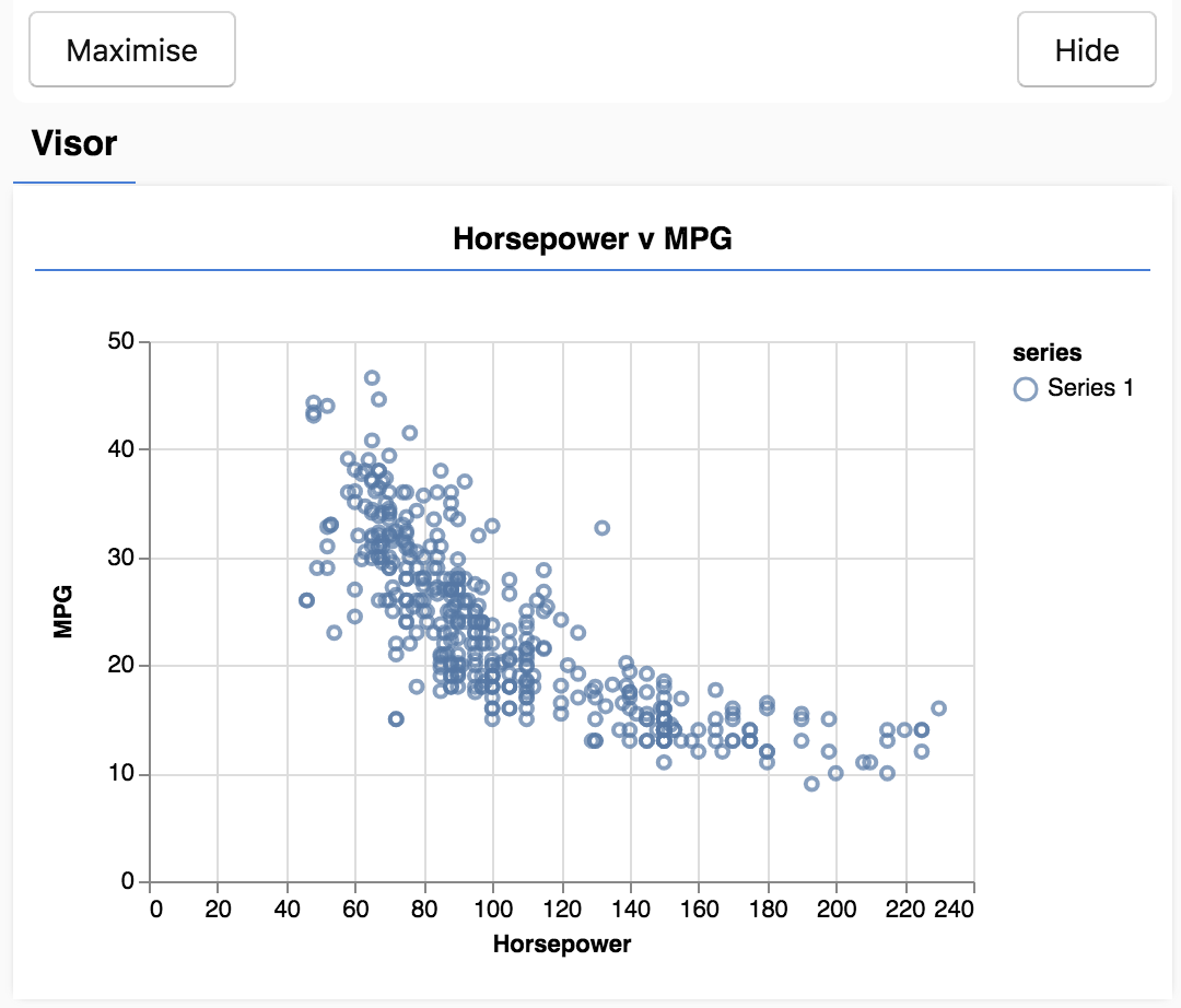
This panel is known as the visor and is provided by tfjs-vis. It provides a convenient place to display visualizations.
Generally when working with data it is a good idea to find ways to take a look at your data and clean it if necessary. In this case, we had to remove certain entries from carsData that didn't have all the required fields. Visualizing the data can give us a sense of whether there is any structure to the data that the model can learn.
We can see from the plot above that there is a negative correlation between horsepower and MPG, i.e. as horsepower goes up, cars generally get fewer miles per gallon.
Conceptualize our task
Our input data will now look like this.
...
{
  "mpg":15,
  "horsepower":165,
},
{
  "mpg":18,
  "horsepower":150,
},
{
  "mpg":16,
  "horsepower":150,
},
...
Our goal is to train a model that will take one number, Horsepower and learn to predict one number, Miles per Gallon. Remember that one-to-one mapping, as it will be important for the next section.
We are going to feed these examples, the horsepower and the MPG, to a neural network that will learn from these examples a formula (or function) to predict MPG given horsepower. This learning from examples for which we have the correct answers is called Supervised Learning.
In this section we will write code to describe the model architecture. Model architecture is just a fancy way of saying "which functions will the model run when it is executing", or alternatively "what algorithm will our model use to compute its answers".
ML models are algorithms that take an input and produce an output. When using neural networks, the algorithm is a set of layers of neurons with ‘weights' (numbers) governing their output. The training process learns the ideal values for those weights.
Add the following function to your script.js file to define the model architecture.
function createModel() {
  // Create a sequential model
  const model = tf.sequential();

  // Add a single input layer
  model.add(tf.layers.dense({inputShape: [1], units: 1, useBias: true}));

  // Add an output layer
  model.add(tf.layers.dense({units: 1, useBias: true}));

  return model;
}
This is one of the simplest models we can define in tensorflow.js, let us break-down each line a bit.
Instantiate the model
const model = tf.sequential();This instantiates a tf.Model object. This model is sequential because its inputs flow straight down to its output. Other kinds of models can have branches, or even multiple inputs and outputs, but in many cases your models will be sequential. Sequential models also have an easier to use API.
Add layers
model.add(tf.layers.dense({inputShape: [1], units: 1, useBias: true}));This adds an input layer to our network, which is automatically connected to a `dense` layer with one hidden unit. A dense layer is a type of layer that multiplies its inputs by a matrix (called weights) and then adds a number (called the bias) to the result. As this is the first layer of the network, we need to define our inputShape. The inputShape is [1] because we have 1 number as our input (the horsepower of a given car).
units sets how big the weight matrix will be in the layer. By setting it to 1 here we are saying there will be 1 weight for each of the input features of the data.
model.add(tf.layers.dense({units: 1}));The code above creates our output layer. We set units to 1 because we want to output 1 number.
Create an instance
Add the following code to the run function we defined earlier.
// Create the model
const model = createModel();
tfvis.show.modelSummary({name: 'Model Summary'}, model);
This will create an instance of the model and show a summary of the layers on the webpage.
To get the performance benefits of TensorFlow.js that make training machine learning models practical, we need to convert our data to tensors. We will also perform a number of transformations on our data that are best practices, namely shuffling and normalization.
Add the following code to your script.js file
/**
 * Convert the input data to tensors that we can use for machine
 * learning. We will also do the important best practices of _shuffling_
 * the data and _normalizing_ the data
 * MPG on the y-axis.
 */
function convertToTensor(data) {
  // Wrapping these calculations in a tidy will dispose any
  // intermediate tensors.

  return tf.tidy(() => {
    // Step 1. Shuffle the data
    tf.util.shuffle(data);

    // Step 2. Convert data to Tensor
    const inputs = data.map(d => d.horsepower)
    const labels = data.map(d => d.mpg);

    const inputTensor = tf.tensor2d(inputs, [inputs.length, 1]);
    const labelTensor = tf.tensor2d(labels, [labels.length, 1]);

    //Step 3. Normalize the data to the range 0 - 1 using min-max scaling
    const inputMax = inputTensor.max();
    const inputMin = inputTensor.min();
    const labelMax = labelTensor.max();
    const labelMin = labelTensor.min();

    const normalizedInputs = inputTensor.sub(inputMin).div(inputMax.sub(inputMin));
    const normalizedLabels = labelTensor.sub(labelMin).div(labelMax.sub(labelMin));

    return {
      inputs: normalizedInputs,
      labels: normalizedLabels,
      // Return the min/max bounds so we can use them later.
      inputMax,
      inputMin,
      labelMax,
      labelMin,
    }
  });
}
Let's break down what's going on here.
Shuffle the data
// Step 1. Shuffle the data
tf.util.shuffle(data);
Here we randomize the order of the examples we will feed to the training algorithm. Shuffling is important because typically during training the dataset is broken up into smaller subsets, called batches, that the model is trained on. Shuffling helps each batch have a variety of data from across the data distribution. By doing so we help the model:
- Not learn things that are purely dependent on the order the data was fed in
- Not be sensitive to the structure in subgroups (e.g. if it only see high horsepower cars for the first half of its training it may learn a relationship that does not apply across the rest of the dataset).
Convert to tensors
// Step 2. Convert data to Tensor
const inputs = data.map(d => d.horsepower)
const labels = data.map(d => d.mpg);

const inputTensor = tf.tensor2d(inputs, [inputs.length, 1]);
const labelTensor = tf.tensor2d(labels, [labels.length, 1]);
Here we make two arrays, one for our input examples (the horsepower entries), and another for the true output values (which are known as labels in machine learning).
We then convert each array data to a 2d tensor. The tensor will have a shape of [num_examples, num_features_per_example]. Here we have inputs.length examples and each example has 1 input feature (the horsepower).
Normalize the data
//Step 3. Normalize the data to the range 0 - 1 using min-max scaling
const inputMax = inputTensor.max();
const inputMin = inputTensor.min();
const labelMax = labelTensor.max();
const labelMin = labelTensor.min();

const normalizedInputs = inputTensor.sub(inputMin).div(inputMax.sub(inputMin));
const normalizedLabels = labelTensor.sub(labelMin).div(labelMax.sub(labelMin));
Next we do another best practice for machine learning training. We normalize the data. Here we normalize the data into the numerical range 0-1 using min-max scaling. Normalization is important because the internals of many machine learning models you will build with tensorflow.js are designed to work with numbers that are not too big. Common ranges to normalize data to include 0 to 1 or -1 to 1. You will have more success training your models if you get into the habit of normalizing your data to some reasonable range.
Return the data and the normalization bounds
return {
  inputs: normalizedInputs,
  labels: normalizedLabels,
  // Return the min/max bounds so we can use them later.
  inputMax,
  inputMin,
  labelMax,
  labelMin,
}
We want to keep the values we used for normalization during training so that we can un-normalize the outputs to get them back into our original scale and to allow us to normalize future input data the same way.
With our model instance created and our data represented as tensors we have everything in place to start the training process.
Copy the following function into your script.js file.
async function trainModel(model, inputs, labels) {
  // Prepare the model for training.
  model.compile({
    optimizer: tf.train.adam(),
    loss: tf.losses.meanSquaredError,
    metrics: ['mse'],
  });

  const batchSize = 32;
  const epochs = 50;

  return await model.fit(inputs, labels, {
    batchSize,
    epochs,
    shuffle: true,
    callbacks: tfvis.show.fitCallbacks(
      { name: 'Training Performance' },
      ['loss', 'mse'],
      { height: 200, callbacks: ['onEpochEnd'] }
    )
  });
}
Let's break this down.
Prepare for training
// Prepare the model for training.
model.compile({
  optimizer: tf.train.adam(),
  loss: tf.losses.meanSquaredError,
  metrics: ['mse'],
});
We have to ‘compile' the model before we train it. To do so, we have to specify a number of very important things:
optimizer: This is the algorithm that is going to govern the updates to the model as it sees examples. There are many optimizers available in TensorFlow.js. Here we have picked the adam optimizer as it is quite effective in practice and requires no configuration.loss: this is a function that will tell the model how well it is doing on learning each of the batches (data subsets) that it is shown. Here we usemeanSquaredErrorto compare the predictions made by the model with the true values.
const batchSize = 32;
const epochs = 50;
Next we pick a batchSize and a number of epochs:
batchSizerefers to the size of the data subsets that the model will see on each iteration of training. Common batch sizes tend to be in the range 32-512. There isn't really an ideal batch size for all problems and it is beyond the scope of this tutorial to describe the mathematical motivations for various batch sizes.epochsrefers to the number of times the model is going to look at the entire dataset that you provide it. Here we will take 50 iterations through the dataset.
Start the train loop
return await model.fit(inputs, labels, {
  batchSize,
  epochs,
  callbacks: tfvis.show.fitCallbacks(
    { name: 'Training Performance' },
    ['loss', 'mse'],
    { height: 200, callbacks: ['onEpochEnd'] }
  )
});
model.fit is the function we call to start the training loop. It is an asynchronous function so we return the promise it gives us so that the caller can determine when training is complete.
To monitor training progress we pass some callbacks to model.fit. We use tfvis.show.fitCallbacks to generate functions that plot charts for the ‘loss' and ‘mse' metric we specified earlier.
Put it all together
Now we have to call the functions we have defined from our run function.
Add the following code to the bottom of your run function.
// Convert the data to a form we can use for training.
const tensorData = convertToTensor(data);
const {inputs, labels} = tensorData;

// Train the model
await trainModel(model, inputs, labels);
console.log('Done Training');
When you refresh the page, after a few seconds you should see the following graphs updating.
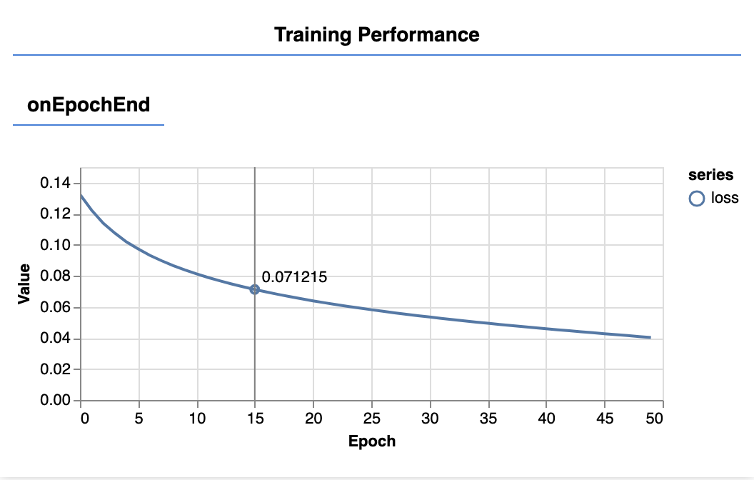
These are created by the callbacks we created earlier. They display the loss and mse, averaged over the whole dataset, at the end of each epoch.
When training a model we want to see the loss go down. In this case, because our metric is a measure of error, we want to see it go down as well.
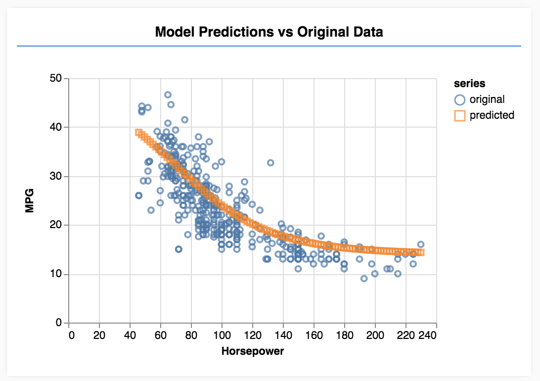
Now that our model is trained, we want to make some predictions. Let's evaluate the model by seeing what it predicts for a uniform range of numbers of low to high horsepowers.
Add the following function to your script.js file
function testModel(model, inputData, normalizationData) {
  const {inputMax, inputMin, labelMin, labelMax} = normalizationData;

  // Generate predictions for a uniform range of numbers between 0 and 1;
  // We un-normalize the data by doing the inverse of the min-max scaling
  // that we did earlier.
  const [xs, preds] = tf.tidy(() => {

    const xs = tf.linspace(0, 1, 100);
    const preds = model.predict(xs.reshape([100, 1]));

    const unNormXs = xs
      .mul(inputMax.sub(inputMin))
      .add(inputMin);

    const unNormPreds = preds
      .mul(labelMax.sub(labelMin))
      .add(labelMin);

    // Un-normalize the data
    return [unNormXs.dataSync(), unNormPreds.dataSync()];
  });


  const predictedPoints = Array.from(xs).map((val, i) => {
    return {x: val, y: preds[i]}
  });

  const originalPoints = inputData.map(d => ({
    x: d.horsepower, y: d.mpg,
  }));


  tfvis.render.scatterplot(
    {name: 'Model Predictions vs Original Data'},
    {values: [originalPoints, predictedPoints], series: ['original', 'predicted']},
    {
      xLabel: 'Horsepower',
      yLabel: 'MPG',
      height: 300
    }
  );
}
A few things to notice in the function above.
const xs = tf.linspace(0, 1, 100);
const preds = model.predict(xs.reshape([100, 1]));
We generate 100 new ‘examples' to feed to the model. Model.predict is how we feed those examples into the model. Note that they need to be have a similar shape ([num_examples, num_features_per_example]) as when we did training.
// Un-normalize the data
const unNormXs = xs
  .mul(inputMax.sub(inputMin))
  .add(inputMin);

const unNormPreds = preds
  .mul(labelMax.sub(labelMin))
  .add(labelMin);
To get the data back to our original range (rather than 0-1) we use the values we calculated while normalizing, but just invert the operations.
return [unNormXs.dataSync(), unNormPreds.dataSync()];.dataSync() is a method we can use to get a typedarray of the values stored in a tensor. This allows us to process those values in regular JavaScript. This is a synchronous version of the .data() method which is generally preferred.
Finally we use tfjs-vis to plot the original data and the predictions from the model.
Add the following code to your run function.
// Make some predictions using the model and compare them to the
// original data
testModel(model, data, tensorData);
Refresh the page and you should see something like the following once the model finishes training.
Congratulations! You have just trained a simple machine learning model. It currently performs what is known as linear regression which tries to fit a line to the trend present in input data.
The steps in training a machine learning model include:
Formulate your task:
- Is it a regression problem or a classification one?
- Can this be done with supervised learning or unsupervised learning?
- What is the shape of the input data? What should the output data look like?
Prepare your data:
- Clean your data and manually inspect it for patterns when possible
- Shuffle your data before using it for training
- Normalize your data into a reasonable range for the neural network. Usually 0-1 or -1-1 are good ranges for numerical data.
- Convert your data into tensors
Build and run your model:
- Define your model using
tf.sequentialortf.modelthen add layers to it usingtf.layers.* - Choose an optimizer (adam is usually a good one), and parameters like batch size and number of epochs.
- Choose an appropriate loss function for your problem, and an accuracy metric to help your evaluate progress.
meanSquaredErroris a common loss function for regression problems. - Monitor training to see whether the loss is going down
Evaluate your model
- Choose an evaluation metric for your model that you can monitor while training. Once it's trained, try making some test predictions to get a sense of prediction quality.
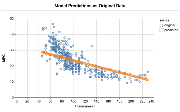
- Experiment changing the number of epochs. How many epochs do you need before the graph flattens out.
- Experiment with increasing the number of units in the hidden layer.
- Experiment with adding more hidden layers in between the first hidden layer we added and the final output layer. The code for these extra layers should look something like this.
model.add(tf.layers.dense({units: 50, activation: 'sigmoid'}));The most important new thing about these hidden layers is that they introduce a non-linear activation function, in this case sigmoid activation. To learn more about activation functions, see this article.
See if you can get the model to produce output like in the image below.