In this tutorial, we'll build a TensorFlow.js model to recognize handwritten digits with a convolutional neural network. First, we'll train the classifier by having it "look" at thousands of handwritten digit images and their labels. Then we'll evaluate the classifier's accuracy using test data that the model has never seen.
This task is considered a classification task as we are training the model to assign a category (the digit that appears in the image) to the input image. We will train the model by showing it many examples of inputs along with the correct output. This is referred to as supervised learning.
What you will build
You will make a webpage that uses TensorFlow.js to train a model in the browser. Given a black and white image of a particular size it will classify which digit appears in the image. The steps involved are:
- Load the data.
- Define the architecture of the model.
- Train the model and monitor its performance as it trains.
- Evaluate the trained model by making some predictions.
What you'll learn
- TensorFlow.js syntax for creating convolutional models using the TensorFlow.js Layers API.
- Formulating classification tasks in TensorFlow.js
- How to monitor in-browser training using the tfjs-vis library.
What you'll need
- A recent version of Chrome or another modern browser that supports ES6 modules.
- A text editor, either running locally on your machine or on the web via something like Codepen or Glitch.
- Knowledge of HTML, CSS, JavaScript, and Chrome DevTools (or your preferred browsers devtools).
- A high level conceptual understanding of Neural Networks. If you need an introduction or refresher, consider watching this video by 3blue1brown or this video on Deep Learning in Javascript by Ashi Krishnan.
You should also be comfortable with the material in our first training tutorial.
Create an HTML page and include the JavaScript
 Copy the following code into an html file called
 index.html
<!DOCTYPE html>
<html>
<head>
  <meta charset="utf-8">
  <meta http-equiv="X-UA-Compatible" content="IE=edge">
  <meta name="viewport" content="width=device-width, initial-scale=1.0">
  <title>TensorFlow.js Tutorial</title>

  <!-- Import TensorFlow.js -->
  <script src="https://cdn.jsdelivr.net/npm/@tensorflow/tfjs@1.0.0/dist/tf.min.js"></script>
  <!-- Import tfjs-vis -->
  <script src="https://cdn.jsdelivr.net/npm/@tensorflow/tfjs-vis@1.0.2/dist/tfjs-vis.umd.min.js"></script>

  <!-- Import the data file -->
  <script src="data.js" type="module"></script>

  <!-- Import the main script file -->
  <script src="script.js" type="module"></script>

</head>

<body>
</body>
</html>
Create the JavaScript files for the data and the code
- In the same folder as the HTML file above, create a file called data.js file and copy the content from this link into that file.
- In the same folder as step one, create a file called script.js and put the following code in it.
console.log('Hello TensorFlow');Test it out
Now that you've got the HTML and JavaScript files created, test them out. Open up the index.html file in your browser and open up the devtools console.
If everything is working, there should be two global variables created. tf is a reference to the TensorFlow.js library, tfvis is a reference to the tfjs-vis library.
You should see a message that says Hello TensorFlow, if so, you are ready to move on to the next step.
In this tutorial you will be training a model to learn to recognize digits in images like the ones below. These images are 28x28px greyscale images from a dataset called MNIST.


We have provided code to load these images from a special sprite file (~10MB) that we have created for you so that we can focus on the training portion.
Feel free to study the data.js file to understand how the data is loaded. Or once you are done with this tutorial, create your own approach to loading the data.
The provided code contains a class MnistData that has two public methods:
nextTrainBatch(batchSize): returns a random batch of images and their labels from the training set.nextTestBatch(batchSize): returns a batch of images and their labels from the test set
The MnistData class also does the important steps of shuffling and normalizing the data.
There are a total of 65,000 images, we will use up to 55,000 images to train the model, saving 10,000 images that we can use to test the model's performance once we are done. And we are going to do all of that in the browser!
Let's load the data and test that it is loaded correctly.
Add the following code to your script.js file.
import {MnistData} from './data.js';

async function showExamples(data) {
  // Create a container in the visor
  const surface =
    tfvis.visor().surface({ name: 'Input Data Examples', tab: 'Input Data'});

  // Get the examples
  const examples = data.nextTestBatch(20);
  const numExamples = examples.xs.shape[0];

  // Create a canvas element to render each example
  for (let i = 0; i < numExamples; i++) {
    const imageTensor = tf.tidy(() => {
      // Reshape the image to 28x28 px
      return examples.xs
        .slice([i, 0], [1, examples.xs.shape[1]])
        .reshape([28, 28, 1]);
    });

    const canvas = document.createElement('canvas');
    canvas.width = 28;
    canvas.height = 28;
    canvas.style = 'margin: 4px;';
    await tf.browser.toPixels(imageTensor, canvas);
    surface.drawArea.appendChild(canvas);

    imageTensor.dispose();
  }
}

async function run() {
  const data = new MnistData();
  await data.load();
  await showExamples(data);
}

document.addEventListener('DOMContentLoaded', run);
Refresh the page and after a few seconds you should see a panel on the left with a number of images.
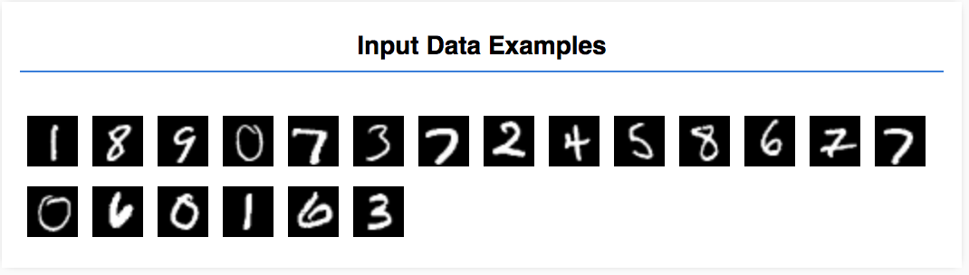
Our input data looks like this.
Our goal is to train a model that will take one image and learn to predict a score for each of the possible 10 classes that image may belong to (the digits 0-9).
Each image is 28px wide 28px high and has a 1 color channel as it is a grayscale image. So the shape of each image is [28, 28, 1].
Remember that we do a one-to-ten mapping, as well as the shape of each input example, since it is important for the next section.
In this section we will write code to describe the model architecture. Model architecture is a fancy way of saying "which functions will the model run when it is executing", or alternatively "what algorithm will our model use to compute its answers".
In machine learning we define an architecture (or algorithm) and let the training process learn the parameters of that algorithm.
Add the following function to your script.js file to define the model architecture
function getModel() {
  const model = tf.sequential();

  const IMAGE_WIDTH = 28;
  const IMAGE_HEIGHT = 28;
  const IMAGE_CHANNELS = 1;

  // In the first layer of our convolutional neural network we have
  // to specify the input shape. Then we specify some parameters for
  // the convolution operation that takes place in this layer.
  model.add(tf.layers.conv2d({
    inputShape: [IMAGE_WIDTH, IMAGE_HEIGHT, IMAGE_CHANNELS],
    kernelSize: 5,
    filters: 8,
    strides: 1,
    activation: 'relu',
    kernelInitializer: 'varianceScaling'
  }));

  // The MaxPooling layer acts as a sort of downsampling using max values
  // in a region instead of averaging.
  model.add(tf.layers.maxPooling2d({poolSize: [2, 2], strides: [2, 2]}));

  // Repeat another conv2d + maxPooling stack.
  // Note that we have more filters in the convolution.
  model.add(tf.layers.conv2d({
    kernelSize: 5,
    filters: 16,
    strides: 1,
    activation: 'relu',
    kernelInitializer: 'varianceScaling'
  }));
  model.add(tf.layers.maxPooling2d({poolSize: [2, 2], strides: [2, 2]}));

  // Now we flatten the output from the 2D filters into a 1D vector to prepare
  // it for input into our last layer. This is common practice when feeding
  // higher dimensional data to a final classification output layer.
  model.add(tf.layers.flatten());

  // Our last layer is a dense layer which has 10 output units, one for each
  // output class (i.e. 0, 1, 2, 3, 4, 5, 6, 7, 8, 9).
  const NUM_OUTPUT_CLASSES = 10;
  model.add(tf.layers.dense({
    units: NUM_OUTPUT_CLASSES,
    kernelInitializer: 'varianceScaling',
    activation: 'softmax'
  }));


  // Choose an optimizer, loss function and accuracy metric,
  // then compile and return the model
  const optimizer = tf.train.adam();
  model.compile({
    optimizer: optimizer,
    loss: 'categoricalCrossentropy',
    metrics: ['accuracy'],
  });

  return model;
}
Let us look at this in a bit more detail.
Convolutions
model.add(tf.layers.conv2d({
  inputShape: [IMAGE_WIDTH, IMAGE_HEIGHT, IMAGE_CHANNELS],
  kernelSize: 5,
  filters: 8,
  strides: 1,
  activation: 'relu',
  kernelInitializer: 'varianceScaling'
}));
Here we are using a sequential model.
We are using a conv2d layer instead of a dense layer. We can't go into all the details of how convolutions work, but here are a few resources that explain the underlying operation:
Let's break down each argument in the configuration object for conv2d:
inputShape. The shape of the data that will flow into the first layer of the model. In this case, our MNIST examples are 28x28-pixel black-and-white images. The canonical format for image data is[row, column, depth], so here we want to configure a shape of[28, 28, 1]. 28 rows and columns for the number of pixels in each dimension, and a depth of 1 because our images have only 1 color channel. Note that we do not specify a batch size in the input shape. Layers are designed to be batch size agnostic so that during inference you can pass a tensor of any batch size in.kernelSize. The size of the sliding convolutional filter windows to be applied to the input data. Here, we set akernelSizeof5, which specifies a square, 5x5 convolutional window.filters. The number of filter windows of sizekernelSizeto apply to the input data. Here, we will apply 8 filters to the data.strides. The "step size" of the sliding window—i.e., how many pixels the filter will shift each time it moves over the image. Here, we specify strides of 1, which means that the filter will slide over the image in steps of 1 pixel.activation. The activation function to apply to the data after the convolution is complete. In this case, we are applying a Rectified Linear Unit (ReLU) function, which is a very common activation function in ML models.kernelInitializer. The method to use for randomly initializing the model weights, which is very important to training dynamics. We won't go into the details of initialization here, butVarianceScaling(used here) is generally a good initializer choice.
Flattening our data representation
model.add(tf.layers.flatten());Images are high dimensional data, and convolution operations tend to increase the size of the data that went into them. Before passing them to our final classification layer we need to flatten the data into one long array. Dense layers (which we use as our final layer) only take `tensor1d`s, so this step is common in many classification tasks.
Compute our final probability distribution
const NUM_OUTPUT_CLASSES = 10;
model.add(tf.layers.dense({
  units: NUM_OUTPUT_CLASSES,
  kernelInitializer: 'varianceScaling',
  activation: 'softmax'
}));
We will use a dense layer with a softmax activation to compute probability distributions over the 10 possible classes. The class with the highest score will be the predicted digit.
Choose an optimizer and loss function
const optimizer = tf.train.adam();
model.compile({
  optimizer: optimizer,
  loss: 'categoricalCrossentropy',
  metrics: ['accuracy'],
});
We compile the model specifying an optimizer, loss function and metrics we want to keep track of.
In contrast to our first tutorial, here we use categoricalCrossentropy as our loss function. As the name implies this is used when the output of our model is a probability distribution. categoricalCrossentropy measures the error between the probability distribution generated by the last layer of our model and the probability distribution given by our true label.
For example if our digit truly represents a 7 we might have the following results
Index | 0 | 1 | 2 | 3 | 4 | 5 | 6 | 7 | 8 | 9 |
True Label | 0 | 0 | 0 | 0 | 0 | 0 | 0 | 1 | 0 | 0 |
Prediction | 0.1 | 0.01 | 0.01 | 0.01 | 0.20 | 0.01 | 0.01 | 0.60 | 0.03 | 0.02 |
Categorical cross entropy will produce a single number indicating how similar the prediction vector is to our true label vector.
The data representation used here for the labels is called one-hot encoding and is common in classification problems. Each class has a probability associated with it for each example. When we know exactly what it should be we can set that probability to 1 and the others to 0. See this page for more information on one-hot encoding.
The other metric we will monitor is accuracy which for a classification problem is the percentage of correct predictions out of all predictions.
Copy the following function to your script.js file.
async function train(model, data) {
  const metrics = ['loss', 'val_loss', 'acc', 'val_acc'];
  const container = {
    name: 'Model Training', styles: { height: '1000px' }
  };
  const fitCallbacks = tfvis.show.fitCallbacks(container, metrics);

  const BATCH_SIZE = 512;
  const TRAIN_DATA_SIZE = 5500;
  const TEST_DATA_SIZE = 1000;

  const [trainXs, trainYs] = tf.tidy(() => {
    const d = data.nextTrainBatch(TRAIN_DATA_SIZE);
    return [
      d.xs.reshape([TRAIN_DATA_SIZE, 28, 28, 1]),
      d.labels
    ];
  });

  const [testXs, testYs] = tf.tidy(() => {
    const d = data.nextTestBatch(TEST_DATA_SIZE);
    return [
      d.xs.reshape([TEST_DATA_SIZE, 28, 28, 1]),
      d.labels
    ];
  });

  return model.fit(trainXs, trainYs, {
    batchSize: BATCH_SIZE,
    validationData: [testXs, testYs],
    epochs: 10,
    shuffle: true,
    callbacks: fitCallbacks
  });
}
Then add the following code to your run function.
const model = getModel();
tfvis.show.modelSummary({name: 'Model Architecture'}, model);

await train(model, data);
Refresh the page and after a few seconds you should see some graphs reporting training progress.
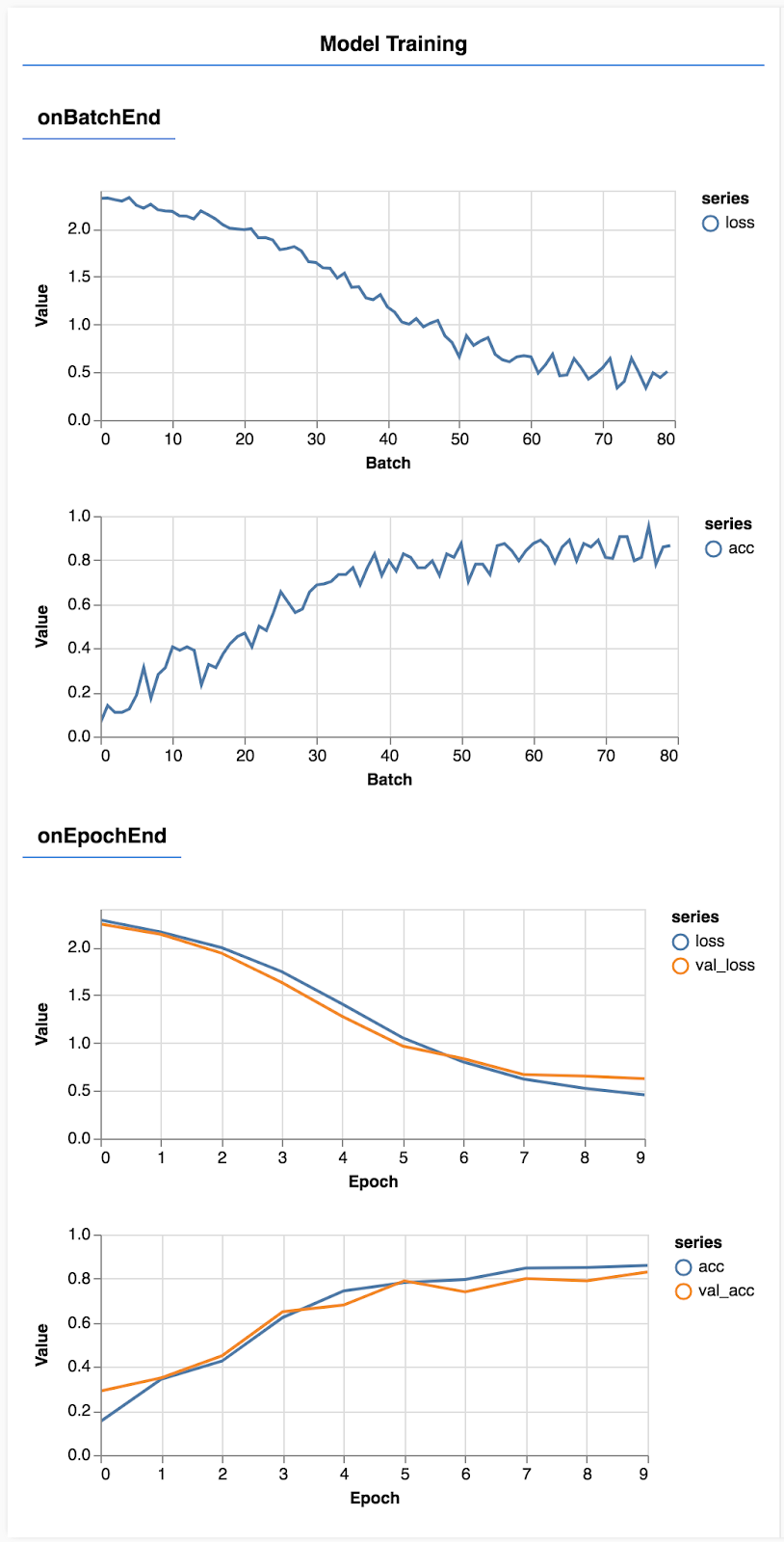
Let's look at that in a bit more detail.
Monitor metrics
const metrics = ['loss', 'val_loss', 'acc', 'val_acc'];Here we decide which metrics we are going to monitor. We will monitor loss and accuracy on the training set as well as loss and accuracy on the validation set (val_loss and val_acc respectively). We'll talk more about the validation set below.
Prepare data as tensors
const BATCH_SIZE = 512;
const TRAIN_DATA_SIZE = 5500;
const TEST_DATA_SIZE = 1000;

const [trainXs, trainYs] = tf.tidy(() => {
  const d = data.nextTrainBatch(TRAIN_DATA_SIZE);
  return [
    d.xs.reshape([TRAIN_DATA_SIZE, 28, 28, 1]),
    d.labels
  ];
});

const [testXs, testYs] = tf.tidy(() => {
  const d = data.nextTestBatch(TEST_DATA_SIZE);
  return [
    d.xs.reshape([TEST_DATA_SIZE, 28, 28, 1]),
    d.labels
  ];
});
Here we make two datasets, a training set that we will train the model on, and a validation set that we will test the model on at the end of each epoch, however the data in the validation set is never shown to the model during training.
The data class we provided makes it easy to get tensors from the image data. But we still reshape the tensors into the shape expected by the model, [num_examples, image_width, image_height, channels], before we can feed these to the model. For each dataset we have both inputs (the Xs) and labels (the Ys).
return model.fit(trainXs, trainYs, {
  batchSize: BATCH_SIZE,
  validationData: [testXs, testYs],
  epochs: 10,
  shuffle: true,
  callbacks: fitCallbacks
});
We call model.fit to start the training loop. We also pass a validationData property to indicate which data the model should use to test itself after each epoch (but not use for training).
If we do well on our training data but not on our validation data, it means the model is likely overfitting to the training data and won't generalize well to input it has not previously seen.
The validation accuracy provides a good estimate on how well our model will do on data it hasn't seen before (as long as that data resembles the validation set in some way). However we may want a more detailed breakdown of performance across the different classes.
There are a couple of methods in tfjs-vis that can help you with this.
Add the following code to the bottom of your script.js file
const classNames = ['Zero', 'One', 'Two', 'Three', 'Four', 'Five', 'Six', 'Seven', 'Eight', 'Nine'];

function doPrediction(model, data, testDataSize = 500) {
  const IMAGE_WIDTH = 28;
  const IMAGE_HEIGHT = 28;
  const testData = data.nextTestBatch(testDataSize);
  const testxs = testData.xs.reshape([testDataSize, IMAGE_WIDTH, IMAGE_HEIGHT, 1]);
  const labels = testData.labels.argMax([-1]);
  const preds = model.predict(testxs).argMax([-1]);

  testxs.dispose();
  return [preds, labels];
}


async function showAccuracy(model, data) {
  const [preds, labels] = doPrediction(model, data);
  const classAccuracy = await tfvis.metrics.perClassAccuracy(labels, preds);
  const container = {name: 'Accuracy', tab: 'Evaluation'};
  tfvis.show.perClassAccuracy(container, classAccuracy, classNames);

  labels.dispose();
}

async function showConfusion(model, data) {
  const [preds, labels] = doPrediction(model, data);
  const confusionMatrix = await tfvis.metrics.confusionMatrix(labels, preds);
  const container = {name: 'Confusion Matrix', tab: 'Evaluation'};
  tfvis.render.confusionMatrix(
      container, {values: confusionMatrix}, classNames);

  labels.dispose();
}
What is this code doing?
- Makes a prediction.
- Computes accuracy metrics.
- Shows the metrics
Let's take a closer look at each step.
Make Predictions
function doPrediction(model, data, testDataSize = 500) {
  const IMAGE_WIDTH = 28;
  const IMAGE_HEIGHT = 28;
  const testData = data.nextTestBatch(testDataSize);
  const testxs = testData.xs.reshape([testDataSize, IMAGE_WIDTH, IMAGE_HEIGHT, 1]);
  const labels = testData.labels.argMax([-1]);
  const preds = model.predict(testxs).argMax([-1]);

  testxs.dispose();
  return [preds, labels];
}
First we need to make some predictions. Here we will make take 500 images and predict what digit is in them (you can increase this number later to test on a larger set of images).
Notably the argmax function is what gives us the index of the highest probability class. Remember that the model outputs a probability for each class. Here we find out the highest probability and assign use that as the prediction.
You may also notice that we can do predictions on all 500 examples at once. This is the power of vectorization that TensorFlow.js provides.
Show per class accuracy
async function showAccuracy() {
  const [preds, labels] = doPrediction();
  const classAccuracy = await tfvis.metrics.perClassAccuracy(labels, preds);
  const container = { name: 'Accuracy', tab: 'Evaluation' };
  tfvis.show.perClassAccuracy(container, classAccuracy, classNames);

  labels.dispose();
}
With a set of predictions and labels we can calculate accuracy for each class.
Show a confusion matrix
async function showConfusion() {
  const [preds, labels] = doPrediction();
  const confusionMatrix = await tfvis.metrics.confusionMatrix(labels, preds);
  const container = { name: 'Confusion Matrix', tab: 'Evaluation' };
  tfvis.render.confusionMatrix(
      container, {values: confusionMatrix}, classNames);

  labels.dispose();
}
A confusion matrix is similar to per class accuracy but further breaks it down to show patterns of misclassification. It allows you to see if the model is getting confused about any particular pairs of classes.
Display the evaluation
Add the following code to the bottom of your run function to show the evaluation.
await showAccuracy(model, data);
await showConfusion(model, data);
You should see a display that looks like the following.
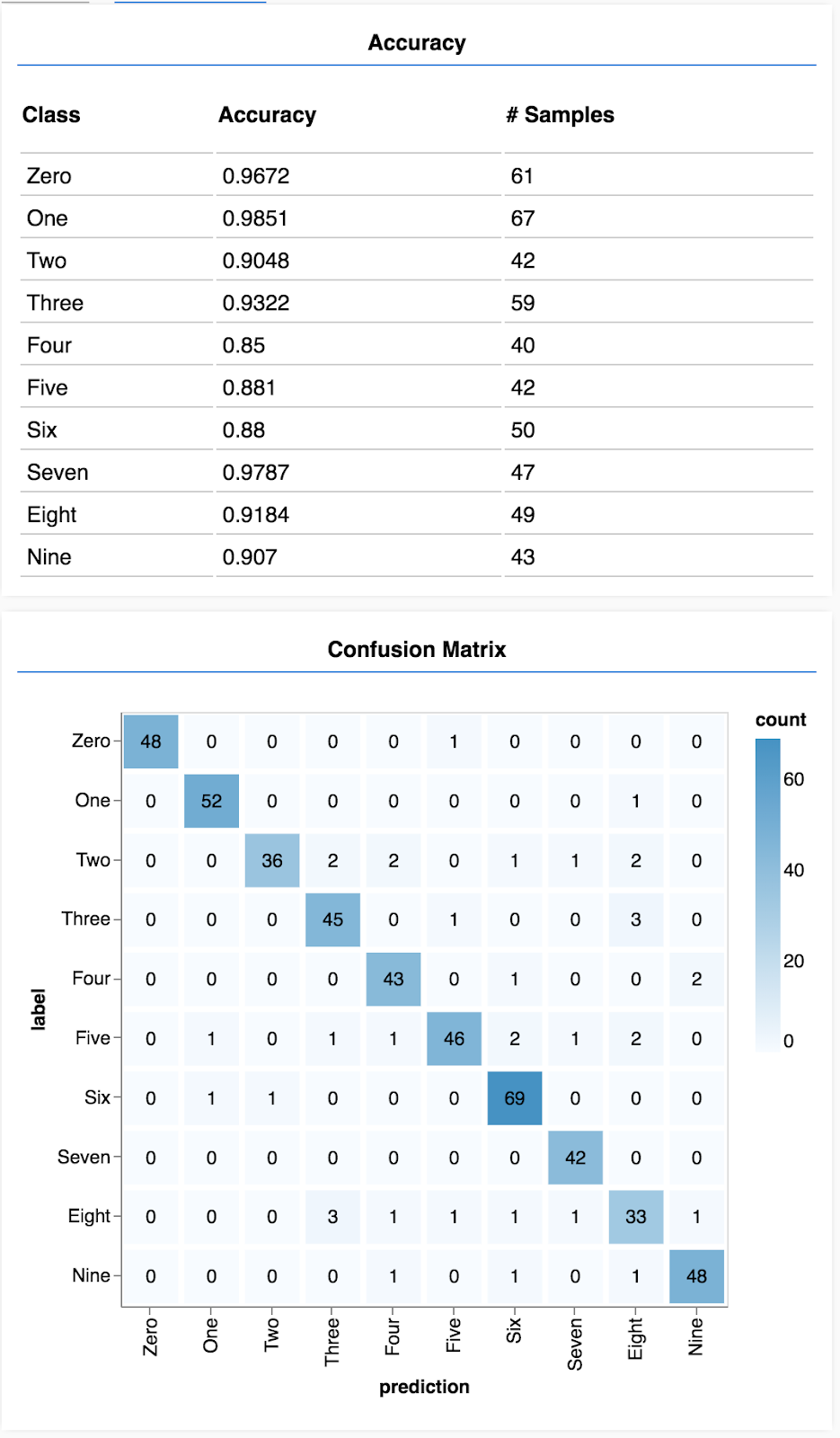
Congratulations! You have just trained a convolutional neural network!
Predicting categories for input data is called a classification task.
Classification tasks require an appropriate data representation for the labels
- Common representations of labels include one-hot encoding of categories
Prepare your data:
- It is useful to keep some data aside that the model never sees during training that you can use to evaluate the model. This is called the validation set.
Build and run your model:
- Convolutional models have been shown to perform well on image tasks.
- Classification problems usually use categorical cross entropy for their loss functions.
- Monitor training to see whether the loss is going down and accuracy is going up.
Evaluate your model
- Decide on some way to evaluate your model once it's trained to see how well it is doing on the initial problem you wanted to solve.
- Per class accuracy and confusion matrices can give you a finer breakdown of model performance than just overall accuracy.