In this codelab you'll use convolutions to classify images of horses and humans. You'll be using TensorFlow in this lab to create a CNN that is trained to recognize images of horses and humans, and classify them.
Prerequisites
If you've never built convolutions with TensorFlow before, you may want to complete Build convolutions and perform pooling codelab, where we introduce convolutions and pooling, and Build convolutional neural networks (CNNs) to enhance computer vision, where we discuss how to make computers more efficient at recognizing images.
What you'll learn
- How to train computers to recognize features in an image in which the subject isn't clear
What you'll build
- A convolutional neural network that can distinguish between pictures of horses and pictures of humans
What you'll need
You can find the code for the rest of the codelab running in Colab.
You'll also need TensorFlow installed, and the libraries you installed in the previous codelab.
You'll do this by building a horses-or-humans classifier that will tell you if a given image contains a horse or a human, where the network is trained to recognize features that determine which is which. You'll have to do some processing of the data before you can train.
First, download the data:
!wget --no-check-certificate https://storage.googleapis.com/laurencemoroney-blog.appspot.com/horse-or-human.zip -O /tmp/horse-or-human.zipThe following Python code will use the OS library to use operating system libraries, giving you access to the file system and the zip file library, therefore allowing you to unzip the data.
import os
import zipfile

local_zip = '/tmp/horse-or-human.zip'
zip_ref = zipfile.ZipFile(local_zip, 'r')
zip_ref.extractall('/tmp/horse-or-human')
zip_ref.close()
The contents of the zip file are extracted to the base directory /tmp/horse-or-human, which contain horses and human subdirectories.
In short, the training set is the data that is used to tell the neural network model that
"this is what a horse looks like" and "this is what a human looks like."
You do not explicitly label the images as horses or humans.
Later you'll see something called an ImageDataGenerator being used. It reads images from subdirectories and automatically labels them from the name of that subdirectory. For example, you have a training directory containing a horses directory and a humans directory. ImageDataGenerator will label the images appropriately for you, reducing a coding step.
Define each of those directories.
# Directory with our training horse pictures
train_horse_dir = os.path.join('/tmp/horse-or-human/horses')

# Directory with our training human pictures
train_human_dir = os.path.join('/tmp/horse-or-human/humans')
Now, see what the filenames look like in the horses and humans training directories:
train_horse_names = os.listdir(train_horse_dir)
print(train_horse_names[:10])
train_human_names = os.listdir(train_human_dir)
print(train_human_names[:10])
Find the total number of horse and human images in the directories:
print('total training horse images:', len(os.listdir(train_horse_dir)))
print('total training human images:', len(os.listdir(train_human_dir)))
Take a look at a few pictures to get a better sense of what they look like.
First, configure the matplot parameters:
%matplotlib inline

import matplotlib.pyplot as plt
import matplotlib.image as mpimg

# Parameters for our graph; we'll output images in a 4x4 configuration
nrows = 4
ncols = 4

# Index for iterating over images
pic_index = 0
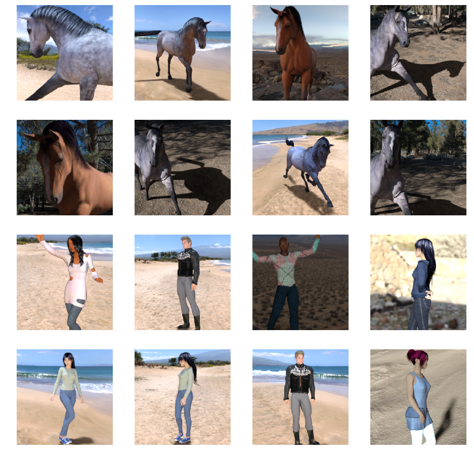
Now, display a batch of eight horse pictures and eight human pictures. You can rerun the cell to see a fresh batch each time.
# Set up matplotlib fig, and size it to fit 4x4 pics
fig = plt.gcf()
fig.set_size_inches(ncols * 4, nrows * 4)

pic_index += 8
next_horse_pix = [os.path.join(train_horse_dir, fname)
                for fname in train_horse_names[pic_index-8:pic_index]]
next_human_pix = [os.path.join(train_human_dir, fname)
                for fname in train_human_names[pic_index-8:pic_index]]

for i, img_path in enumerate(next_horse_pix+next_human_pix):
  # Set up subplot; subplot indices start at 1
  sp = plt.subplot(nrows, ncols, i + 1)
  sp.axis('Off') # Don't show axes (or gridlines)

  img = mpimg.imread(img_path)
  plt.imshow(img)

plt.show()
Here are some example images showing horses and humans in different poses and orientations:
Start defining the model.
Begin by importing TensorFlow:
import tensorflow as tfThen, add convolutional layers and flatten the final result to feed into the densely connected layers. Finally, add the densely connected layers.
Note that because you're facing a two-class classification problem (a binary classification problem) you'll end your network with a sigmoid activation so that the output of your network will be a single scalar between 0 and 1, encoding the probability that the current image is class 1 (as opposed to class 0).
model = tf.keras.models.Sequential([
    # Note the input shape is the desired size of the image 300x300 with 3 bytes color
    # This is the first convolution
    tf.keras.layers.Conv2D(16, (3,3), activation='relu', input_shape=(300, 300, 3)),
    tf.keras.layers.MaxPooling2D(2, 2),
    # The second convolution
    tf.keras.layers.Conv2D(32, (3,3), activation='relu'),
    tf.keras.layers.MaxPooling2D(2,2),
    # The third convolution
    tf.keras.layers.Conv2D(64, (3,3), activation='relu'),
    tf.keras.layers.MaxPooling2D(2,2),
    # The fourth convolution
    tf.keras.layers.Conv2D(64, (3,3), activation='relu'),
    tf.keras.layers.MaxPooling2D(2,2),
    # The fifth convolution
    tf.keras.layers.Conv2D(64, (3,3), activation='relu'),
    tf.keras.layers.MaxPooling2D(2,2),
    # Flatten the results to feed into a DNN
    tf.keras.layers.Flatten(),
    # 512 neuron hidden layer
    tf.keras.layers.Dense(512, activation='relu'),
    # Only 1 output neuron. It will contain a value from 0-1 where 0 for 1 class ('horses') and 1 for the other ('humans')
    tf.keras.layers.Dense(1, activation='sigmoid')
])
The model.summary() method call prints a summary of the network.
model.summary()You can see the results here:
Layer (type)                 Output Shape              Param #
=================================================================
conv2d (Conv2D)              (None, 298, 298, 16)      448
_________________________________________________________________
max_pooling2d (MaxPooling2D) (None, 149, 149, 16)      0
_________________________________________________________________
conv2d_1 (Conv2D)            (None, 147, 147, 32)      4640
_________________________________________________________________
max_pooling2d_1 (MaxPooling2 (None, 73, 73, 32)        0
_________________________________________________________________
conv2d_2 (Conv2D)            (None, 71, 71, 64)        18496
_________________________________________________________________
max_pooling2d_2 (MaxPooling2 (None, 35, 35, 64)        0
_________________________________________________________________
conv2d_3 (Conv2D)            (None, 33, 33, 64)        36928
_________________________________________________________________
max_pooling2d_3 (MaxPooling2 (None, 16, 16, 64)        0
_________________________________________________________________
conv2d_4 (Conv2D)            (None, 14, 14, 64)        36928
_________________________________________________________________
max_pooling2d_4 (MaxPooling2 (None, 7, 7, 64)          0
_________________________________________________________________
flatten (Flatten)            (None, 3136)              0
_________________________________________________________________
dense (Dense)                (None, 512)               1606144
_________________________________________________________________
dense_1 (Dense)              (None, 1)                 513
=================================================================
Total params: 1,704,097
Trainable params: 1,704,097
Non-trainable params: 0
The output shape column shows how the size of your feature map evolves in each successive layer. The convolution layers reduce the size of the feature maps by a bit due to padding and each pooling layer halves the dimensions.
Next, configure the specifications for model training. Train your model with the binary_crossentropy loss because it's a binary classification problem and your final activation is a sigmoid. (For a refresher on loss metrics, see Descending into ML.) Use the rmsprop optimizer with a learning rate of 0.001. During training, monitor classification accuracy.
from tensorflow.keras.optimizers import RMSprop

model.compile(loss='binary_crossentropy',
              optimizer=RMSprop(lr=0.001),
              metrics=['acc'])
Set up data generators that read pictures in your source folders, convert them to float32 tensors, and feed them (with their labels) to your network.
You'll have one generator for the training images and one for the validation images. Your generators will yield batches of images of size 300x300 and their labels (binary).
As you may already know, data that goes into neural networks should usually be normalized in some way to make it more amenable to processing by the network. (It's uncommon to feed raw pixels into a CNN.) In your case, you'll preprocess your images by normalizing the pixel values to be in the [0, 1] range (originally all values are in the [0, 255] range).
In Keras, that can be done via the keras.preprocessing.image.ImageDataGenerator class using the rescale parameter. That ImageDataGenerator class allows you to instantiate generators of augmented image batches (and their labels) via .flow(data, labels) or .flow_from_directory(directory). Those generators can then be used with the Keras model methods that accept data generators as inputs: fit_generator, evaluate_generator and predict_generator.
from tensorflow.keras.preprocessing.image import ImageDataGenerator

# All images will be rescaled by 1./255
train_datagen = ImageDataGenerator(rescale=1./255)

# Flow training images in batches of 128 using train_datagen generator
train_generator = train_datagen.flow_from_directory(
        '/tmp/horse-or-human/',  # This is the source directory for training images
        target_size=(300, 300),  # All images will be resized to 150x150
        batch_size=128,
        # Since we use binary_crossentropy loss, we need binary labels
        class_mode='binary')
Train for 15 epochs. (That may take a few minutes to run.)
history = model.fit_generator(
      train_generator,
      steps_per_epoch=8,
      epochs=15,
      verbose=1)
Note the values per epoch.
The Loss and Accuracy are a great indication of progress of training. It's making a guess as to the classification of the training data, and then measuring it against the known label, calculating the result. Accuracy is the portion of correct guesses.
Epoch 1/15
9/9 [==============================] - 9s 1s/step - loss: 0.8662 - acc: 0.5151
Epoch 2/15
9/9 [==============================] - 8s 927ms/step - loss: 0.7212 - acc: 0.5969
Epoch 3/15
9/9 [==============================] - 8s 921ms/step - loss: 0.6612 - acc: 0.6592
Epoch 4/15
9/9 [==============================] - 8s 925ms/step - loss: 0.3135 - acc: 0.8481
Epoch 5/15
9/9 [==============================] - 8s 919ms/step - loss: 0.4640 - acc: 0.8530
Epoch 6/15
9/9 [==============================] - 8s 896ms/step - loss: 0.2306 - acc: 0.9231
Epoch 7/15
9/9 [==============================] - 8s 915ms/step - loss: 0.1464 - acc: 0.9396
Epoch 8/15
9/9 [==============================] - 8s 935ms/step - loss: 0.2663 - acc: 0.8919
Epoch 9/15
9/9 [==============================] - 8s 883ms/step - loss: 0.0772 - acc: 0.9698
Epoch 10/15
9/9 [==============================] - 9s 951ms/step - loss: 0.0403 - acc: 0.9805
Epoch 11/15
9/9 [==============================] - 8s 891ms/step - loss: 0.2618 - acc: 0.9075
Epoch 12/15
9/9 [==============================] - 8s 902ms/step - loss: 0.0434 - acc: 0.9873
Epoch 13/15
9/9 [==============================] - 8s 904ms/step - loss: 0.0187 - acc: 0.9932
Epoch 14/15
9/9 [==============================] - 9s 951ms/step - loss: 0.0974 - acc: 0.9649
Epoch 15/15
9/9 [==============================] - 8s 877ms/step - loss: 0.2859 - acc: 0.9338
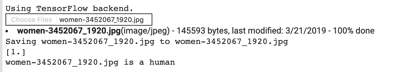
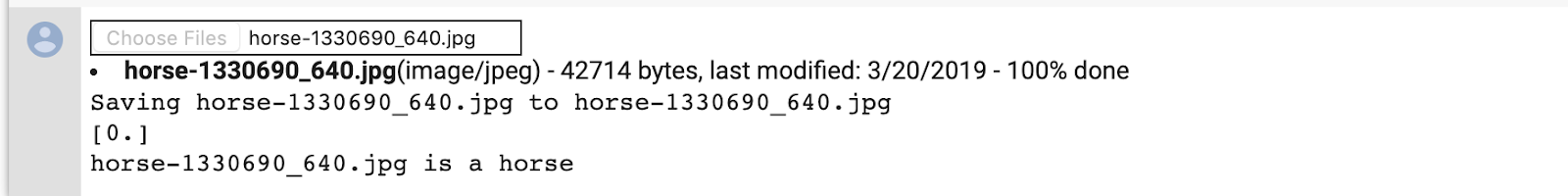
Now actually run a prediction using the model. The code will allow you to choose one or more files from your file system. It will then upload them and run them through the model, giving an indication of whether the object is a horse or a human.
You can download images from the internet to your file system to try them out! Note that you might see that the network makes a lot of mistakes despite the fact that the training accuracy is above 99%.
That's due to something called overfitting, which means that the neural network is trained with very limited data (there are only roughly 500 images of each class). So it's very good at recognizing images that look like those in the training set, but it can fail a lot at images that are not in the training set.
That's a datapoint proving that the more data that you train on, the better your final network will be!
There are many techniques that can be used to make your training better, despite limited data, including something called image augmentation, but that's beyond the scope of this codelab.
import numpy as np
from google.colab import files
from keras.preprocessing import image

uploaded = files.upload()

for fn in uploaded.keys():

  # predicting images
  path = '/content/' + fn
  img = image.load_img(path, target_size=(300, 300))
  x = image.img_to_array(img)
  x = np.expand_dims(x, axis=0)

  images = np.vstack([x])
  classes = model.predict(images, batch_size=10)
  print(classes[0])
  if classes[0]>0.5:
    print(fn + " is a human")
  else:
    print(fn + " is a horse")
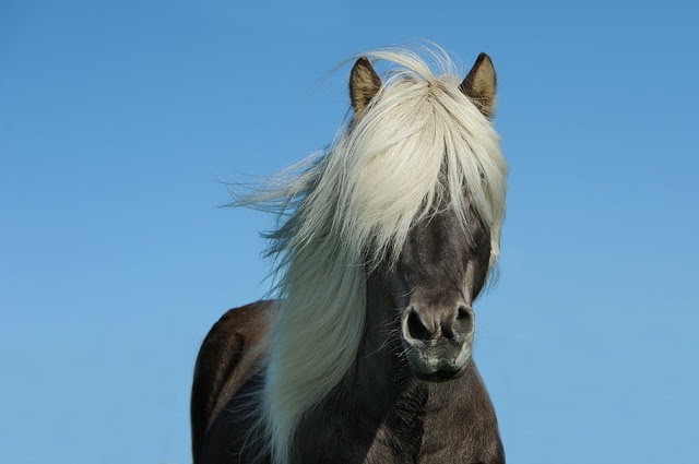
For example, say that you want to test with this image:

Here's what the colab produces:
Despite it being a cartoon graphic, it still classifies correctly.
The following image also classifies correctly:
Try some images of your own and explore!
To get a feel for what kind of features your CNN has learned, a fun thing to do is visualize how an input gets transformed as it goes through the CNN.
Pick a random image from the training set, then generate a figure where each row is the output of a layer and each image in the row is a specific filter in that output feature map. Rerun that cell to generate intermediate representations for a variety of training images.
import numpy as np
import random
from tensorflow.keras.preprocessing.image import img_to_array, load_img

# Let's define a new Model that will take an image as input, and will output
# intermediate representations for all layers in the previous model after
# the first.
successive_outputs = [layer.output for layer in model.layers[1:]]
#visualization_model = Model(img_input, successive_outputs)
visualization_model = tf.keras.models.Model(inputs = model.input, outputs = successive_outputs)
# Let's prepare a random input image from the training set.
horse_img_files = [os.path.join(train_horse_dir, f) for f in train_horse_names]
human_img_files = [os.path.join(train_human_dir, f) for f in train_human_names]
img_path = random.choice(horse_img_files + human_img_files)

img = load_img(img_path, target_size=(300, 300))  # this is a PIL image
x = img_to_array(img)  # Numpy array with shape (150, 150, 3)
x = x.reshape((1,) + x.shape)  # Numpy array with shape (1, 150, 150, 3)

# Rescale by 1/255
x /= 255

# Let's run our image through our network, thus obtaining all
# intermediate representations for this image.
successive_feature_maps = visualization_model.predict(x)

# These are the names of the layers, so can have them as part of our plot
layer_names = [layer.name for layer in model.layers]

# Now let's display our representations
for layer_name, feature_map in zip(layer_names, successive_feature_maps):
  if len(feature_map.shape) == 4:
    # Just do this for the conv / maxpool layers, not the fully-connected layers
    n_features = feature_map.shape[-1]  # number of features in feature map
    # The feature map has shape (1, size, size, n_features)
    size = feature_map.shape[1]
    # We will tile our images in this matrix
    display_grid = np.zeros((size, size * n_features))
    for i in range(n_features):
      # Postprocess the feature to make it visually palatable
      x = feature_map[0, :, :, i]
      x -= x.mean()
      x /= x.std()
      x *= 64
      x += 128
      x = np.clip(x, 0, 255).astype('uint8')
      # We'll tile each filter into this big horizontal grid
      display_grid[:, i * size : (i + 1) * size] = x
    # Display the grid
    scale = 20. / n_features
    plt.figure(figsize=(scale * n_features, scale))
    plt.title(layer_name)
    plt.grid(False)
    plt.imshow(display_grid, aspect='auto', cmap='viridis')
Here are example results:
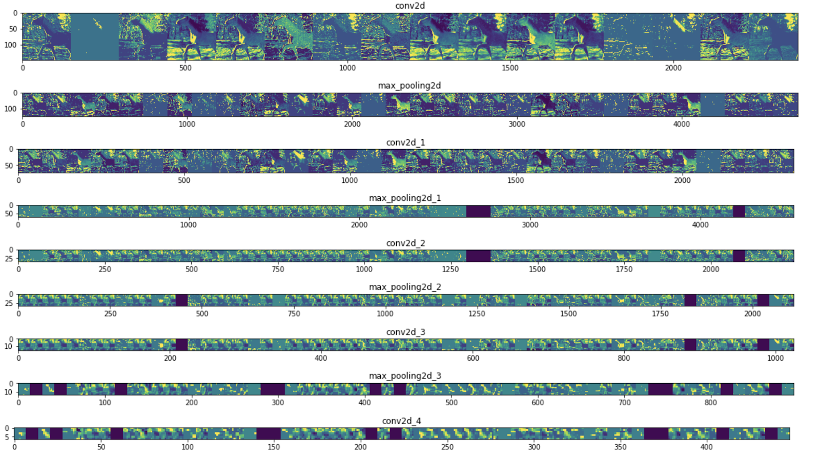
As you can see, you go from the raw pixels of the images to increasingly abstract and compact representations. The representations downstream start highlighting what the network pays attention to, and they show fewer and fewer features being "activated." Most are set to zero. That's called sparsity. Representation sparsity is a key feature of deep learning.
Those representations carry increasingly less information about the original pixels of the image, but increasingly refined information about the class of the image. You can think of a CNN (or a deep network in general) as an information distillation pipeline.
You've learned to use CNNs to enhance complex images. To learn how to further enhance your computer vision models, proceed to Use convolutional neural networks (CNNs) with large datasets to avoid overfitting.