In this codelab, you'll create a computer vision model that can recognize items of clothing with TensorFlow.
Prerequisites
- A solid knowledge of Python
- Basic programming skills
What you'll learn
In this codelab, you'll:
- Train a neural network to recognize articles of clothing
- Complete a series of exercises to guide you through experimenting with the different layers of the network
What you'll build
- A neural network that identifies articles of clothing
What you'll need
If you've never created a neural network for computer vision with TensorFlow, you can use Colaboratory, a browser-based environment containing all the required dependencies. You can find the code for the rest of the codelab running in Colab.
Otherwise, the main language that you'll use for training models is Python, so you'll need to install it. In addition to that, you'll also need TensorFlow and the NumPy library. You can learn more about and install TensorFlow here. Install NumPy here.
First, walk through the executable Colab notebook.
Start by importing TensorFlow.
import tensorflow as tf
print(tf.__version__)
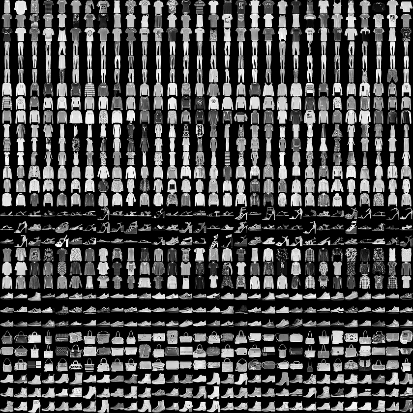
You'll train a neural network to recognize items of clothing from a common dataset called Fashion MNIST. It contains 70,000 items of clothing in 10 different categories. Each item of clothing is in a 28x28 grayscale image. You can see some examples here:

The labels associated with the dataset are:
Label | Description |
0 | T-shirt/top |
1 | Trouser |
2 | Pullover |
3 | Dress |
4 | Coat |
5 | Sandal |
6 | Shirt |
7 | Sneaker |
8 | Bag |
9 | Ankle boot |
The Fashion MNIST data is available in the tf.keras.datasets API. Load it like this:
mnist = tf.keras.datasets.fashion_mnistCalling load_data on that object gives you two sets of two lists: training values and testing values, which represent graphics that show clothing items and their labels.
(training_images, training_labels), (test_images, test_labels) = mnist.load_data()What do those values look like? Print a training image and a training label to see.
You can experiment with different indices in the array.
import matplotlib.pyplot as plt
plt.imshow(training_images[0])
print(training_labels[0])
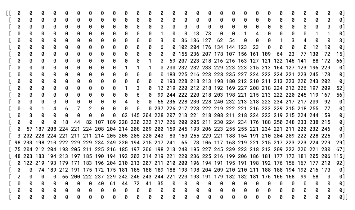
print(training_images[0])
The print of the data for item 0 looks like this:

You'll notice that all the values are integers between 0 and 255. When training a neural network, it's easier to treat all values as between 0 and 1, a process called normalization. Fortunately, Python provides an easy way to normalize a list like that without looping.
training_images  = training_images / 255.0
test_images = test_images / 255.0
You may also want to look at 42, a different boot than the one at index 0.
Now, you might be wondering why there are two datasets—training and testing.
The idea is to have one set of data for training and another set of data that the model hasn't yet encountered to see how well it can classify values. After all, when you're done, you'll want to use the model with data that it hadn't previously seen! Also, without separate testing data, you'll run the risk of the network only memorizing its training data without generalizing its knowledge.
Now design the model. You'll have three layers. Go through them one-by-one and explore the different types of layers and the parameters used for each.
model = tf.keras.models.Sequential([tf.keras.layers.Flatten(),
                                    tf.keras.layers.Dense(128, activation=tf.nn.relu),
tf.keras.layers.Dense(10, activation=tf.nn.softmax)])Sequentialdefines a sequence of layers in the neural network.Flattentakes a square and turns it into a one-dimensional vector.Denseadds a layer of neurons.Activationfunctions tell each layer of neurons what to do. There are lots of options, but use these for now:Relueffectively means that if X is greater than 0 return X, else return 0. It only passes values of 0 or greater to the next layer in the network.Softmaxtakes a set of values, and effectively picks the biggest one. For example, if the output of the last layer looks like [0.1, 0.1, 0.05, 0.1, 9.5, 0.1, 0.05, 0.05, 0.05], then it saves you from having to sort for the largest value—it returns [0,0,0,0,1,0,0,0,0].
Now that the model is defined, the next thing to do is build it. Create a model by first compiling it with an optimizer and loss function, then train it on your training data and labels. The goal is to have the model figure out the relationship between the training data and its training labels. Later, you want your model to see data that resembles your training data, then make a prediction about what that data should look like.
Notice the use of metrics= as a parameter, which allows TensorFlow to report on the accuracy of the training against the test set. It measures how many were right and wrong, and reports the results.
model.compile(optimizer = tf.keras.optimizers.Adam(),
              loss = 'sparse_categorical_crossentropy',
              metrics=['accuracy'])

model.fit(training_images, training_labels, epochs=5)
When model.fit executes, you'll see loss and accuracy:
Epoch 1/5
60000/60000 [=======] - 6s 101us/sample - loss: 0.4964 - acc: 0.8247
Epoch 2/5
60000/60000 [=======] - 5s 86us/sample - loss: 0.3720 - acc: 0.8656
Epoch 3/5
60000/60000 [=======] - 5s 85us/sample - loss: 0.3335 - acc: 0.8780
Epoch 4/5
60000/60000 [=======] - 6s 103us/sample - loss: 0.3134 - acc: 0.8844
Epoch 5/5
60000/60000 [=======] - 6s 94us/sample - loss: 0.2931 - acc: 0.8926
When the model is done training, you will see an accuracy value at the end of the final epoch. It might look something like 0.8926 as above. This tells you that your neural network is about 89% accurate in classifying the training data. In other words, it figured out a pattern match between the image and the labels that worked 89% of the time. Not great, but not bad considering it was only trained for five epochs and done quickly.
How would the model perform on data it hasn't seen? That's why you have the test set. You call model.evaluate and pass in the two sets, and it reports the loss for each. Give it a try:
model.evaluate(test_images, test_labels)And here's the output:
10000/10000 [=====] - 1s 56us/sample - loss: 0.3365 - acc: 0.8789
[0.33648381242752073, 0.8789]
That example returned an accuracy of .8789, meaning it was about 88% accurate. (You might have slightly different values.)
As expected, the model is not as accurate with the unknown data as it was with the data it was trained on! As you learn more about TensorFlow, you'll find ways to improve that.
To explore further, try the exercises in the next step.
Exercise 1
For this first exercise, run the following code:
classifications = model.predict(test_images)
print(classifications[0])
It creates a set of classifications for each of the test images, then prints the first entry in the classifications. The output after you run it is a list of numbers. Why do you think that is and what do those numbers represent?
Try running print(test_labels[0]) and you'll get a 9. Does that help you understand why the list looks the way it does?
The output of the model is a list of 10 numbers. Those numbers are a probability that the value being classified is the corresponding label. For example, the first value in the list is the probability that the clothing is of class 0 and the next is a 1. Notice that they are all very low probabilities except one. Also, because of Softmax, all the probabilities in the list sum to 1.0.
The list and the labels are 0 based, so the ankle boot having label 9 means that it is the 10th of the 10 classes. The list having the 10th element being the highest value means that the neural network has predicted that the item it is classifying is most likely an ankle boot.
Exercise 2
Look at the layers in your model. Experiment with different values for the dense layer with 512 neurons.
What different results do you get for loss and training time? Why do you think that's the case?
For example, if you increase to 1,024 neurons, you have to do more calculations, slowing down the process. But in this case they have a good impact because the model is more accurate. That doesn't mean more is always better. You can hit the law of diminishing returns very quickly.
Exercise 3
What would happen if you remove the Flatten() layer. Why do you think that's the case?
You get an error about the shape of the data. The details of the error may seem vague right now, but it reinforces the rule of thumb that the first layer in your network should be the same shape as your data. Right now your data is 28x28 images, and 28 layers of 28 neurons would be infeasible, so it makes more sense to flatten that 28,28 into a 784x1.
Instead of writing all the code, add the Flatten() layer at the beginning. When the arrays are loaded into the model later, they'll automatically be flattened for you.
Exercise 4
Consider the final (output) layers. Why are there 10 of them? What would happen if you had a different amount than 10?
Try training the network with 5. You get an error as soon as it finds an unexpected value. Another rule of thumb—the number of neurons in the last layer should match the number of classes you are classifying for. In this case, it's the digits 0 through 9, so there are 10 of them, and hence you should have 10 neurons in your final layer.
Exercise 5
Consider the effects of additional layers in the network. What will happen if you add another layer between the one with 512 and the final layer with 10?
There isn't a significant impact because this is relatively simple data. For far more complex data, extra layers are often necessary.
Exercise 6
Before you trained, you normalized the data, going from values that were 0 through 255 to values that were 0 through 1. What would be the impact of removing that? Here's the complete code to give it a try (note that the two lines that normalize the data are commented out).
Why do you think you get different results? There's a great answer here on Stack Overflow.
import tensorflow as tf
print(tf.__version__)
mnist = tf.keras.datasets.fashion_mnist
(training_images, training_labels), (test_images, test_labels) = mnist.load_data()
#training_images=training_images/255.0
#test_images=test_images/255.0
model = tf.keras.models.Sequential([
  tf.keras.layers.Flatten(),
  tf.keras.layers.Dense(512, activation=tf.nn.relu),
  tf.keras.layers.Dense(10, activation=tf.nn.softmax)
])
model.compile(optimizer='adam', loss='sparse_categorical_crossentropy')
model.fit(training_images, training_labels, epochs=5)
model.evaluate(test_images, test_labels)
classifications = model.predict(test_images)
print(classifications[0])
print(test_labels[0])
Earlier, when you trained for extra epochs, you had an issue where your loss might change. It might have taken a bit of time for you to wait for the training to do that and you might have thought that it'd be nice if you could stop the training when you reach a desired value, such as 95% accuracy. If you reach that after 3 epochs, why sit around waiting for it to finish a lot more epochs?
Like any other program, you have callbacks! See them in action:
import tensorflow as tf

class myCallback(tf.keras.callbacks.Callback):
  def on_epoch_end(self, epoch, logs={}):
    if(logs.get('accuracy')>0.95):
      print("\nReached 95% accuracy so cancelling training!")
      self.model.stop_training = True

callbacks = myCallback()
mnist = tf.keras.datasets.fashion_mnist
(training_images, training_labels), (test_images, test_labels) = mnist.load_data()
training_images=training_images/255.0
test_images=test_images/255.0
model = tf.keras.models.Sequential([
  tf.keras.layers.Flatten(),
  tf.keras.layers.Dense(512, activation=tf.nn.relu),
  tf.keras.layers.Dense(10, activation=tf.nn.softmax)
])
model.compile(optimizer='adam', loss='sparse_categorical_crossentropy', metrics=['accuracy'])
model.fit(training_images, training_labels, epochs=5, callbacks=[callbacks])
You've built your first computer vision model! To learn how to enhance your computer vision models, proceed to Build convolutions and perform pooling.